The method and the data
I have already written about the Taylor rule in a quite extensive blog post:
http://macrothoughts.weebly.com/blog/monetary-policy-rules-vs-discretion-and-some-thoughts-about-the-taylor-rule
I have argued that Central Banks should not strictly follow the rule but that they should also use a variety of other indicators (such as TIPS spreads, asset prices, or nominal GDP data) to guide their policy decisions. Nonetheless, I have now calculated the Taylor rule for a set of Eurozone countries because it can be useful indicator of the stance of monetary policy. As a reminder, the Taylor determines how a Central Bank should set the nominal interest, given the economy’s output gap (deviation of actual GDP from potential GDP) and the deviation of inflation from the Central Banks’ inflation target.
Mathematically, the Taylor rule can be expressed as follows:
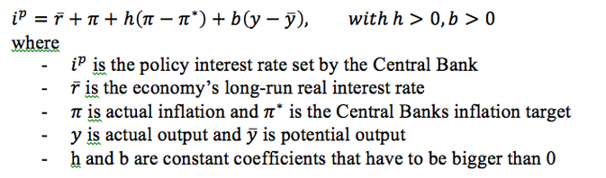
At the time of invention, John Taylor prescribed that the Central Bank should put equal emphasis on the output gap and on inflation deviations from the inflation target. Consequently, the coefficients h and b should both equal to 0.5. The real interest rate in the U.S. was roughly 2% at that time.
I have calculated the Taylor rule for Austria, France, Germany, Ireland and Spain for the period of 1996 to 2013. Similar to John Taylor, I have set the coefficients h and b to 0.5, meaning that the Central Bank is equally concerned about the output gap and the ‘inflation gap’ (deviation from target). I have used the CPI (consumer price index) from the OECD database and the ECB’s inflation target of 2% to calculate the inflation gap for each country. Instead of determining the output gap myself, I have simply used output gap data from the IMF.
Contrary to Taylor, I have not used a real interest rate r of 2%. There are a lot of factors, some of them related to ‘secular stagnation’, that have led to a significant decrease of global real interest rates. These factors include, for example:
- Excess savings and disproportionate accumulation of foreign reserves in South-East Asia.
- Insufficient aggregate demand in most industrialized countries, including the three most important economies in terms of size: the U.S., the Eurozone and Japan.
- A significant reduction in investments in most industrialized countries.
- Slowing population growth in most industrialized countries.
According to a paper published by the IMF, the average global real interest rate has been around 3.3% in between 1996 and 2000. It subsequently fell to about 2.1% for the period of 2001 and 2007. With the outbreak of the financial crisis, the global real interest rate has averaged about 0.6% in between 2008 and 2012. For the year 2013, I have simply assumed the same real interest rate 0f 0.6%.
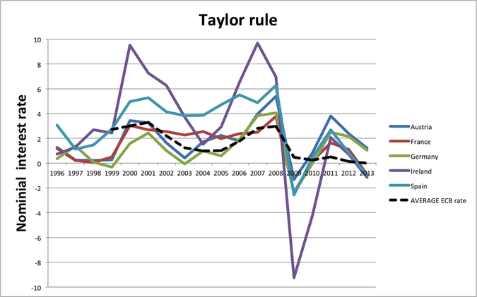
The graph below depicts the Taylor for the set of Eurozone countries mentioned above. I also inserted the nominal interest set by the ECB for comparison. Obviously, the ECB interest rate only starts in 1999 when the euro was introduced. Since I have used annual data throughout, I calculated the ‘average ECB rate’ for any given year. So if the ECB had an interest rate of 1.25% during the first half of the year and then an interest of 0.75% during the second half, this leads to an ‘average ECB rate’ of 1%. One should be aware that in some years the ECB changed its interest rate more frequently whereas in other years it did not change it at all. The decision to calculate a yearly average is somewhat arbitrary. It is nonetheless very useful since for all countries I also calculated the difference between the interest rate prescribed by the Taylor rule and the rate set by the ECB.
I have calculated the Taylor rule for Austria, France, Germany, Ireland and Spain for the period of 1996 to 2013. Similar to John Taylor, I have set the coefficients h and b to 0.5, meaning that the Central Bank is equally concerned about the output gap and the ‘inflation gap’ (deviation from target). I have used the CPI (consumer price index) from the OECD database and the ECB’s inflation target of 2% to calculate the inflation gap for each country. Instead of determining the output gap myself, I have simply used output gap data from the IMF.
Contrary to Taylor, I have not used a real interest rate r of 2%. There are a lot of factors, some of them related to ‘secular stagnation’, that have led to a significant decrease of global real interest rates. These factors include, for example:
- Excess savings and disproportionate accumulation of foreign reserves in South-East Asia.
- Insufficient aggregate demand in most industrialized countries, including the three most important economies in terms of size: the U.S., the Eurozone and Japan.
- A significant reduction in investments in most industrialized countries.
- Slowing population growth in most industrialized countries.
According to a paper published by the IMF, the average global real interest rate has been around 3.3% in between 1996 and 2000. It subsequently fell to about 2.1% for the period of 2001 and 2007. With the outbreak of the financial crisis, the global real interest rate has averaged about 0.6% in between 2008 and 2012. For the year 2013, I have simply assumed the same real interest rate 0f 0.6%.
The graph below depicts the Taylor for the set of Eurozone countries mentioned above. I also inserted the nominal interest set by the ECB for comparison. Obviously, the ECB interest rate only starts in 1999 when the euro was introduced. Since I have used annual data throughout, I calculated the ‘average ECB rate’ for any given year. So if the ECB had an interest rate of 1.25% during the first half of the year and then an interest of 0.75% during the second half, this leads to an ‘average ECB rate’ of 1%. One should be aware that in some years the ECB changed its interest rate more frequently whereas in other years it did not change it at all. The decision to calculate a yearly average is somewhat arbitrary. It is nonetheless very useful since for all countries I also calculated the difference between the interest rate prescribed by the Taylor rule and the rate set by the ECB.
Implications of the Taylor rule analysis
1) During almost the entire time period analyzed, the interest rates for the 5 Eurozone countries prescribed by the Taylor rule move in the same direction, i.e. they rise together and they fall together most of the time. This suggests that the business cycle for the Eurozone countries is to some extent synchronized. Output gaps and inflation deviations seem to be somewhat correlated.
2) The graph also suggests that the Eurozone was a very bad idea in the first place. The Eurozone countries are so diverse that monetary policy is highly inappropriate for some member countries at any point in time. In 2000, for example, the Taylor rule prescribed an interest rate of about 9.5% for Ireland and only 1.6% for Germany while the actual ECB rate was at about 3%. This means that monetary policy was highly expansionary for Ireland, causing an enormous economic boom and a gigantic housing bubble. At the same time, monetary policy was somewhat contractionary for Germany, leading to unnecessary unemployment and slower economic growth.
3) The interest rate prescribed by the Taylor rule for Spain and Ireland increased quite significantly after 1999. This is indicative of the fact that the introduction of the euro led to a substantial economic boom in the European periphery countries. Indeed, the stance of monetary policy for Ireland and Spain was highly inappropriate, in their case far too expansionary, during the entire time period from 1999 up to 2009. It is very plausible that easy money was a strong contributor to the housing bubble that developed in these countries. If one were to do a similar analysis for Greece and Portugal, one would certainly find similar results.
4) The ECB’s monetary policy has been highly contractionary for all Eurozone countries ever since 2009. Indeed, the Taylor rule prescribed mostly large negative nominal interest rates, especially for the crisis countries Spain and Ireland. This is of course not possible because of the zero lower bound. However, one should note that the ECB has only reduced its interest rate to 0 in 2012, 4 years after the outbreak of the crisis. Indeed, the ECB even raised interest rates twice prematurely, thus being one the main culprits of the current economic stagnation in the Eurozone, which by now is worse than the economic performance during the Great Depression in the 1930s!
5) By looking at the graph, one can easily see that monetary policy by the ECB has been much more inappropriate for some countries (e.g. Ireland) than for others (e.g. France). Indeed, the ‘inappropriateness’ of monetary policy is quantifiable by calculating the difference between the interest rate prescribed by the Taylor rule and the actual ECB rate for each year. Below I have calculated this difference for each country from 1999 onwards. According to the rule, a positive deviation means that monetary policy was too easy whereas a negative deviation indicates that monetary policy was too tight in a given year.
Taylor rule deviations, table 1
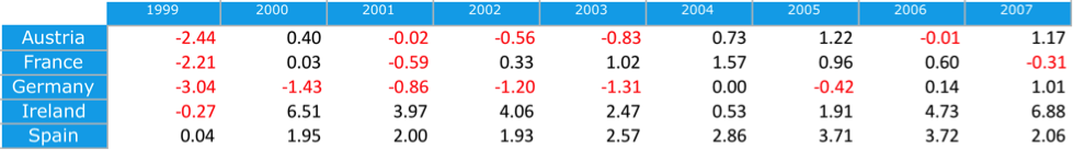
Taylor rule deviations, table 2
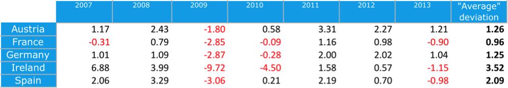
The tables above illustrate that Spain and especially Ireland have indeed experienced the highest ‘Taylor rule deviations’, meaning that the stance of monetary policy was highly inappropriate for these countries most of the time.
It is meaningless to take an average of the deviations since some of them are positive while others are negative. For example, if the ECB rate were at 2% for two years and the Taylor rule prescribed an interest rate of 3% in year 1 and 1% in year 2, then the average of the deviations is equal to 0: [(3-2)+(1-2)]/2
However, this problem is easily resolved by taking the absolute value of all the deviations, thus transforming the negative deviations into positive numbers. I have then taken then average of all absolute values from 1999 to 2013 (see last column in table 2). The result is quite striking. One can see that the stance of monetary policy was the most appropriate for France, closely followed by Germany and Austria whereas it was highly inappropriate for Spain and even more so for Ireland.
Indeed, the interest rate prescribed by the Taylor rule for Ireland deviated, on average, by about 3.5 percentage points from the rate set by the ECB. Meanwhile, the average deviation (of absolute values) for Germany was only 1.25 percentage points, thus roughly a third.
Monetary policy was thus highly inappropriate for countries like Spain and Ireland ever since the creation of the Eurozone. Before the crisis, money was too easy leading to unsustainable economic booms and housing bubbles. Ever since 2009, money has been far too tight, leading to economic depression in Southern Europe. Germany’s enormous influence within the ECB has meant that monetary policy by the European Central Bank has been catered to the needs of the German economy, leaving aside the requirements of other Eurozone countries. This is, of course, highly problematic. Economic stagnation in the Eurozone will last if the ECB continues to implement the tight monetary policy that is requested by the German government and the Bundesbank.

 RSS Feed
